
Introduction
Today, when such beautiful frameworks as Keras, Tensorflow, SkLearn exist, many people are not worried about how Neural Network models work and train. However, when interested people start to dig and search for explanations, they usually face unreasonably significant amounts of linear algebra thrown right into the face without any practical information.
At least, it was my case. Decided to understand Neural Networks, I enrolled in a local university online course. I watched lecture after lecture, noted everything necessary, and from the bottom of my heart waited for practical information and possible algorithms implementation.
The course ended, and I was left with a thick notebook of linear algebra, calculus, and no understanding of what can I do with all this information.
However, I don’t want somebody else to walk on the same road as me, so I decided to write this article. e.g. “Hello, world” in Neural Nets.
Side note: in this guide, I will not explore deeply program architecture and good Python practices as it is not the primary purpose of the article.
Single neurone: what is it?
We find a line that approximates our points the best. The line can be described by the following equation:
By adjusting and we can make our line the best fit for the current points distribution.
And that’s actually what every single neuron in basic Neural Net does. The big difference is that line of best fit presented on the image is in 2D. In the real world, algorithms solve problems in multidimensional space.
For example, if you would like to predict who survives after the Titanic tragedy, you could take into account such parameters as age, fare, sex, number of siblings, etc. See that we already have 4 dimensions to work with. However, you should not be scared of that. A lot of concepts that work in 3D or 2D can also be applied to multidimensional space.
Classification problem
Let’s continue to work on the Titanic survival chance problem and imagine that our neuron already knows the line of best fit. The problem of binary dependent variable classification (survived/did not survive) names Logistic Regression.
The problem is that line is not limited, but probability can’t be lower than zero and higher than one. Here comes a sigmoid function.
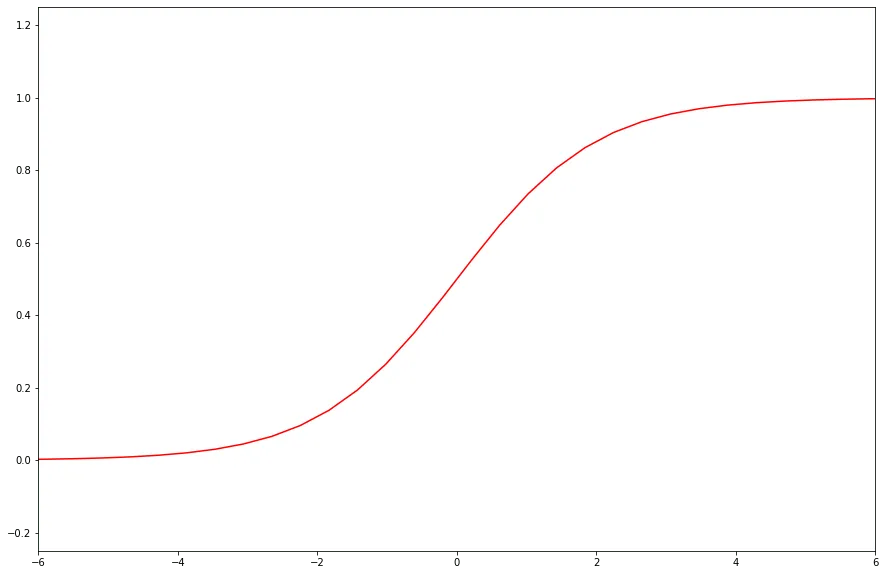
As you see, the function is limited by 0 and 1. So, we will use it to adjust the neuron output. The name of the function that sets neuron output basing on a linear part is an “activation function”.
How this works with multidimensions
The same problem is a little bit different when has multiple dimensions – vector. Then, every component has a different effect on the final result, so also should be a vector.
Formula in vector form:
We set as column-vector and as column-vector. Therefore, to get scalar, we transpose the vector. How it works:
If you feel a little bit uncomfortable with the expression above, repeat basic matrix multiplication.
That's it. This is how a single basic neuron works. It takes input, multiplies it by , adds (just a number), applies activation function, and sends computed value further. This process is named forward propagation. Now, let's implement this in code.
Forward propagation in code
I will use NumPy for basic operations. Of course, you can implement matrix multiplication, addition, etc. by yourself, but NumPy does it more effectively and faster as it’s already compiled.
import numpy as npSigmoid function:
def sigmoid(z):
    return 1 / (1 + np.exp(-z))
Forward propagation function:
def forward_propagation(w, b, x):
    z = np.dot(w.T, x) + b # np.dot(..., ...) — matrix multiplication
    return sigmoid(z)
Great. Now we can calculate forward propagation of a single neuron. But how we figure out and values?
Loss function
To understand how well our algorithm performs, we need to define a loss function. For purposes of binary classification <strong>logarithmic loss</strong> performs well. So, we will use it.
That's how it looks:
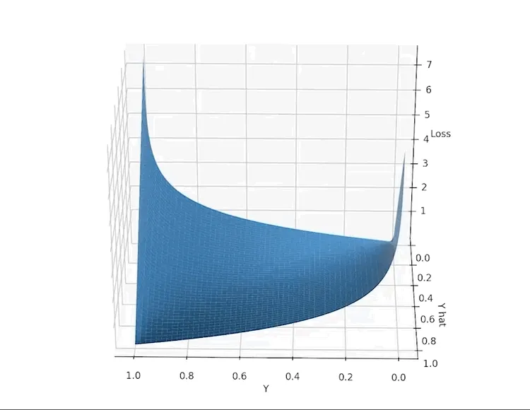
represents computed value, – actual
def loss(A, Y):
    return -(Y * np.log(A) + (1 - Y) * np.log(1 - A))
As you see, loss tends to infinity when and are different, but it's 0 when they are exactly the same.
To train model, we use labeled information: pairs of . represents input vector and – desired output for this vector. If we stack all available into a single matrix, we'll create – a matrix that contains all training data. We can do the same thing for
If we have samples and every x vector is -dimensional, then we can calculate the cost of the algorithm with selected and .
def cost(A, Y, m):
    return 1 / m * np.sum(loss(A, Y))
Vectorization
Currently, we can calculate forward propagation for single (x, y) set and we need to calculate values for all available training pairs. The most obvious answer is to start the for loop and calculate iteratively. But this is not the optimal case. We can use and matrices to calculate forward propagation for the entire training set. That's how it works:
As you see, every row represents forward propagation for every training set.
This approach optimizes code and speeds up calculations. Whenever possible, vectorize code. The same technique can be applied during backpropagation.
In the core of learning: Backpropagation
At this moment we can calculate neuron output and estimate how close it to the actual value. But how we can figure out and values? Here comes a Gradient Descent concept.
The best explanation of GradDescent I ever heard:
It’s like you are trying to find a door in a completely dark room and you can only “feel” in what direction to move
Imagine that you have some function, but you do not know it’s expression. And shape. And you are in multidimensional space. Then, you randomly placed at some point of this function and asked to find its minimum. Not the most pleasant situation, right? However, you know how your position was calculated, so you can find a derivative. But what derivative gives? Let’s take a look at this function.
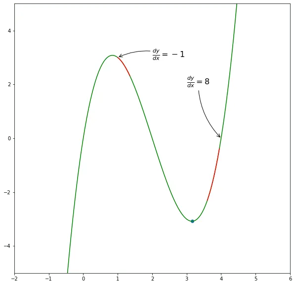
Using derivative we can find direction to the function’s minimum. That’s how it looks animated:
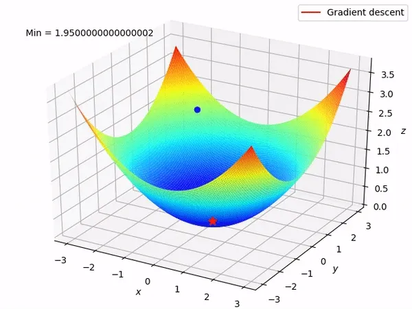
We can take steps in an outlined direction and finally reach a minimum loss point. That’s how we can implement this to adjust and
Where is a learning rate. You can view derivative calculation in the spoiler, here are final expressions:
Do not worry. It all looks a lot better in code. Further, I will use a different notation: as , as , etc. Also, it’s common to name as because it represents activation function value.
dZ = A - Y
db = 1 / m * np.sum(dZ)
dw = 1 / m * np.dot(X, dZ.T)
Then, single back propagation step can be represented in this function:
def backpropagation(w, b, X, A, Y, learning_rate, m):
    dZ = A - Y
    db = 1 / m * np.sum(dZ)
    dw = 1 / m * np.dot(X, dZ.T)
    assert(dw.shape == w.shape)
    w = w - learning_rate * dw
    b = b - learning_rate * db
    return w, b
Initialization
To adjust and , we need to have starting point. We are going to initialise and with zeros
Initialisation:
w = np.zeros((n, 1))
b = np.zeros((n, 1))
Finally, we can write full neuron learning code.
def model(X, Y, learning_rate=0.1, n_iter=2000, costIter = [[],[]]):
    m = X.shape[1]
    n = X.shape[0]
    w = np.zeros((n, 1))
    b = 0
    for i in range(n_iter):
        A = forwardpropagation(w, b, X)
        c = cost(A, Y, m)
        if i % 5 == 0:
            print("Iteration %s: %s" % (i, c))
        costIter[0].append(i)
        costIter[1].append(c)
        w, b = backpropagation(w, b, X, A, Y, learning_rate, m)
    return w, b
In this code, we combine all previous steps:
- Initialize all parameters
- Start a loop
- Perform forward propagation
- Calculate cost
- Print some data / save into array
- Perform backpropagation step and update parameters
Finally, the model returns optimal and values so that we can use them to predict answers for new values.
Testing
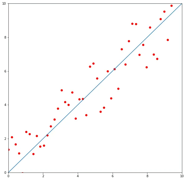
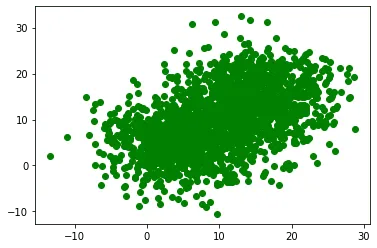
For testing, I selected a line
Let points above the line be blue and ones that below – red. Here is the set that I gave to the model for training.
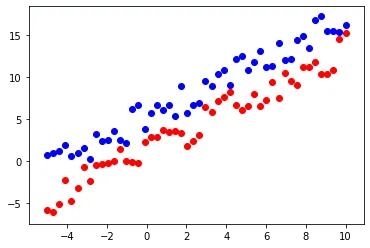
Training:
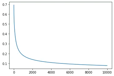
As we see, the cost minimizes overtime. That means that backpropagation works correctly and our and are adjusted right.
To check how well the algorithm performs, I randomly generated 2000 points and requested neuron to classify them.
That’s how the algorithm performed. The green line represents the actual line.
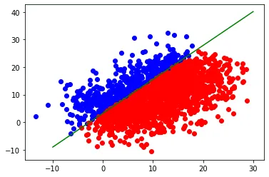
The accuracy is around 99%. I suppose it misclassified ~1% due to the points that lie directly on the line.
What’s special about this classifier?
So one neuron approximates some linear function. How can it distinct cats from dogs, survived from not survived?
By combining neuron in stacks and in layers, we form complicated linear functions compositions, and then we can approximate sophisticated multidimensional functions that find subtle dependencies and relations during training.
But single neuron and backpropagation concept lie in the heart of the whole process.