Flash Attention is a revolutionary technique that dramatically accelerates the attention mechanism in transformer-based models, delivering processing speeds many times faster than naive methods. By cleverly tiling data and minimizing memory transfers, it tackles the notorious GPU memory bottleneck that large language models often struggle with.
In this post, we’ll dive into how Flash Attention leverages efficient I/O-awareness to reduce overhead, then take it a step further by crafting a block-sparse attention kernel in Triton.
What is Attention?
The attention mechanism (or scaled dot-product attention) is a core element of transformer models, which is a leading architecture for solving the problem of language modeling. All popular models, like GPT, LLaMA, and BERT, rely on attention.
The formula is pretty simple:
$$\text{Attention}(Q, K, V) = \text{softmax}\left(\frac{QK^T}{\sqrt{d_k}}\right)V,\\Q, K, V\;—\; \text{query, key, value tensors}$$
The rest is history.
Even though the formula looks simple, its computation involves multiplications of large tensors and a lot of data movement. Considering that this is a core part of the transformer architecture, optimizing the algorithm greatly improves the performance of the model in general.
In the naive implementation, attention requires \(O(n^2)\) additional memory and \(O(n^2)\) compute time complexity, where \(n\) is the sequence length. That's a lot!
Flash Attention
Core Idea
The main idea of Flash attention can be summarized in a simple quote from the original paper:
We argue that a missing principle is making attention algorithms IO-aware — accounting for reads and writes between levels of GPU memory.
That is, modern GPUs have several types of memory:
- SRAM — fast, on-chip, small
- HBM — slower than SRAM, large size. That's what we usually address as GPU memory.
Check out the memory hierarchy in the image below to see the differences in bandwidth and sizes of different memory types.
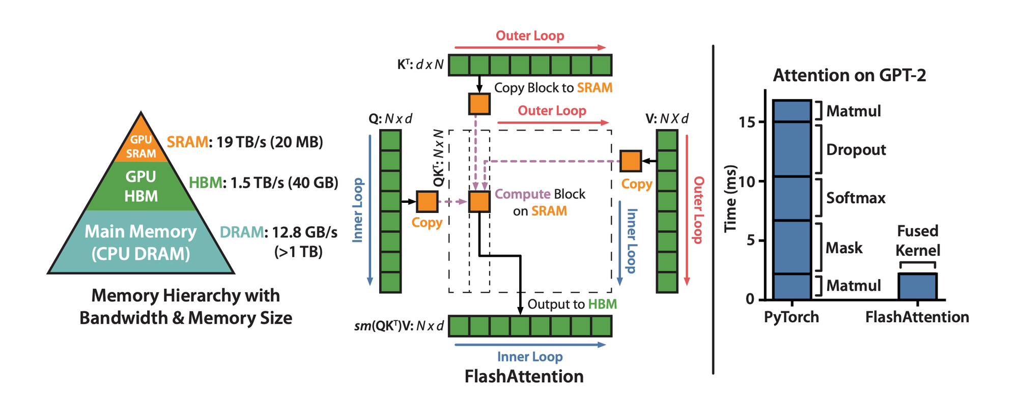
The Flash Attention algorithm proposes a method of computing attention in tiles, without explicitly materializing the attention scores tensor:
$$\text{AttentionScores}(Q, K) = \text{Softmax}\left(\frac{QK^T}{\sqrt{d_k}}\right)$$
It's easy to see that this matrix requires \(O(n^2)\) of memory to store. For large sequence lengths, that's a lot of data! So, if we manage to avoid explicitly materializing this matrix, we can save lots of memory.
However, this matrix is necessary for transformer training as it is a part of backpropagation and gradient calculation. The authors propose that it's better to recalculate this matrix during the backward pass (again without explicit materialization). Not only does this saves lots of memory, but it also provides huge speedups as we don't need to transfer this enormous matrix between different GPU memory types.
Overall, such an approach did not only speed up calculations by taking GPU I/O specifics into account, but also allowed processing huge sequence lengths as memory complexity drops to \(O(n)\).
Tiled Attention Calculation
The last thing to understand is how to compute attention in tiles. Basically, this means that we will calculate attention over the full sequence by processing incoming tokens in small portions.
Well, it's easy to calculate \(QK^T\) in tiles. Considering that attention dimension is not high, we can load full matrix rows and columns and conduct multiplication in tiles.
As dimensions are usually quite small even for enormous models, this limitation is fair.
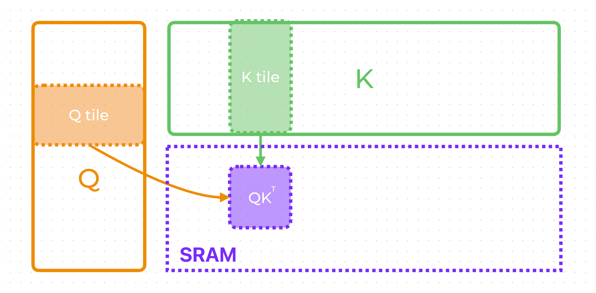
So, we have \(QK^T\) calculated in SRAM. All that's left is to apply softmax, multiply by \(V\), and that's it!
$$\text{Softmax}(z_i) = \frac{e^{z_{i}}}{\sum_{j=1}^T e^{z_{j}}} \; \; \text{for}\; i = 1, 2,\ldots, T$$
That's where the trick is.
The problem is that the softmax denominator requires aggregation over the sequence length to normalize scores, and we do not have access to the whole length as we load data in tiles.
To address it, we can implement a concatenated softmax algorithm. Using it, we can calculate softmax "in batch" mode: by adjusting computed values with the new incoming data.
Taking the algorithm from the original article, we can define rules to compute the softmax over data concatenation. Having two vectors \(x^{(1)}\) and \(x^{(2)}\), we need to calculate the softmax denominator \(l(x)\) over those vectors' concatenation: \(x = \left[x^{(1)}, x^{(2)}\right]\). If the vector's maximum is \(m(x)\), we can easily derive the softmax denominator of the concatenation:
$$m(x) = m\left(\left[x^{(1)}, x^{(2)}\right]\right) = m(m(x^{(1)}), m(x^{(2)})),$$
$$l(x) = l\left(\left[x^{(1)}, x^{(2)}\right]\right) = e^{m(x^{(1)}) - m(x)}l(x^{(1)}) + e^{m(x^{(2)}) - m(x)}l(x^{(2)}).$$
The last equivalence can be easily verified as \(l(x)=\sum_{j=1}^{T} e^{x_{j}}.\)
So, now we have what we want — we can calculate softmax per-tile and then, by doing re-normalization from the formula above, compute the global softmax. The last thing to do is to incorporate the tile of the \(V\) tensor and keep doing the same re-normalization (as matrix multiplication is a linear operation).
And all of this without loading the full sequence into memory or materializing \(QK^T\)!
Also, in the actual algorithm for numerical stability, we will compute not \(\text{Softmax}(x)\) but \(\text{Softmax}(x - \max(x))\). We can do that as softmax is invariant to constant shifts.
Triton Implementation
Now, we can easily implement the outlined algorithm in Triton, which is a tool that allows us to write efficient GPU kernels with the ease of Python.

Outlining the Algorithm
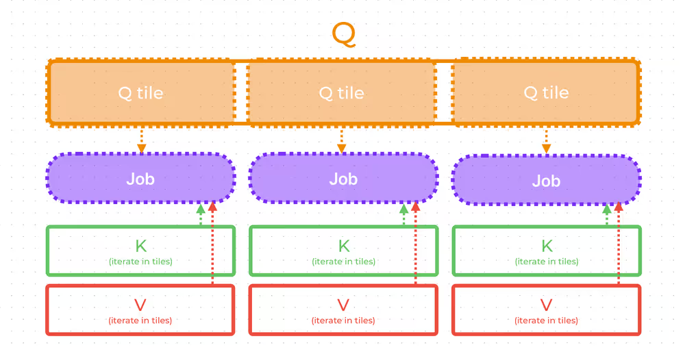
The first step is to decide how we will assign jobs and what data each job will load. By the algorithm of tiled softmax, each job must have access to \(K, V\) over the whole sequence length. So, each job will iterate over \(K, V\) in tiles. We don't have any algorithmic restriction on the number of \(Q\) tiles processed. Therefore, each job will load just one \(Q\) tile and work with it only — this way we will maximize job parallelism.
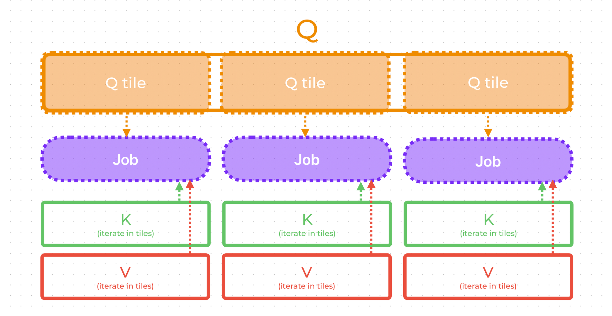
In summary, each job will load a single \(Q\) tile, iterate over all tiles in \(K\) and \(V\), and store one tile of result corresponding to the \(Q\) tile.
The Kernel
What's left is to write the actual code. Let's focus on the core part first, and only then we'll add Triton-specific boilerplates.
Below is a Triton pseudocode with every line explained.
def self_attn_fwd(...):
    # loading sample len
    seq_len = ...

    # running qk^T max (initialized by -inf)
    m_i = tl.zeros([TILE_Q_SIZE], dtype=tl.float32) - float("inf")

    # current softmax denominator
    l_i = tl.zeros([TILE_Q_SIZE], dtype=tl.float32)

    # result tile
    # we will accumulate here (softmax numerator) @ V
    # then, we will divide it by softmax denominator in the very end
    acc = tl.zeros([TILE_Q_SIZE, HEAD_DIM], dtype=tl.float32)

    # notice: we accumulate all values above
    # in fp32 for higher precision

    # account for variable length of samples in batch
    q_tile_indices = q_token_idx + tl.arange(0, TILE_Q_SIZE)
    q_lens_mask = (
        q_tile_indices[:, None] < seq_len
    )

    # loading q tile into SRAM, shape (TILE_Q_SIZE, HEAD_DIM)
    q_tile = ...

    # softmax scale, multiplying by log_2(e)
    # to use faster exp2(...) instead of exp(...)
    softmax_scale: tl.constexpr = tl.cast(SM_SCALE * log_2(e), q_tile.dtype)

    # indices of tokens inside kv tile
    tile_k_arange = tl.arange(0, TILE_K_SIZE)

    # iterate over all tiles in k, v
    for kv_tile_idx in tl.range(
        0, tl.cdiv(seq_len, TILE_K_SIZE), num_stages=PIPELINING
    ):
        # index of the first token in the kv tile
        kv_token_idx = kv_tile_idx * TILE_K_SIZE

        kt_tile = ... # load into SRAM K^T tile no. kv_tile_idx
        v_tile = ... # load into SRAM V tile no. kv_tile_idx

        # compute tile of QK^T
        qk = tl.dot(
            q_tile * softmax_scale,
            kt_tile,
            input_precision=INPUT_PRECISION,
            out_dtype=tl.float32
        )

        # masking out kv tokens after the sequence length
        kv_indices = kv_token_idx + tile_k_arange
        mask = q_lens_mask & (
            kv_indices[None, :] < seq_len
        )

        # set masked out values to -inf
        # for softmax to ignore them
        qk = tl.where(mask, qk, tl.cast(-float("inf"), qk.dtype))

        # calculating new maximum over seq len
        # m(x) = m(m(x1), m(x2))
        m_ij = tl.maximum(m_i, tl.max(qk, 1))

        # e^(x2 - m(x))
        p = tl.math.exp2(qk - m_ij[:, None])

        # current tile softmax denominator
        l_ij = tl.sum(p, 1)

        # from softmax formula: e^(m(x1) - m(x))
        alpha = tl.math.exp2(m_i - m_ij)

        # updating denominator using the formula
        # l(x) = e^(m(x1) - m(x)) * l(x1) + e^(0)l(x2)
        # notice: e^(0) as we subtract m(x) from x2 above
        l_i = l_i * alpha + l_ij

        # update previous acc to address maximum change
        # as e^(xi - m(x1)) * alpha = e^(xi - m(x))
        acc = acc * alpha[:, None]

        # multiply p by v and adding to acc
        acc += tl.dot(
            p.to(v_tile.dtype),
            v_tile,
            input_precision=INPUT_PRECISION,
            out_dtype=tl.float32,
        )

        # storing new maximum
        m_i = m_ij

    # finally incorporate softmax denominator
    acc = acc / l_i[:, None]

    # set fully masked token values to 0 to avoid garbage values
    # in the result
    acc = tl.where(q_lens_mask, acc, 0.0)

    # save the result
    tl.save(acc, ...)
See? Easy!
What's important is that you can see how simple it is to write such a thing as soon as we understand the idea of tiled softmax. Apart from that, there's nothing complicated from the algorithm perspective.
This pseudocode is pretty close to the actual code. You may find it in my GitHub by following the link. All that I added is just data management and PyTorch wrappers.
The code above was extensively tested to match PyTorch's scaled_dot_product_attention. You can also check out the tests to see how to use the written kernel.
Benchmarking
While we wrote the kernel in Triton to improve the algorithm understanding, it's interesting to compare the performance with a naive implementation and PyTorch's scaled_dot_product_attention.
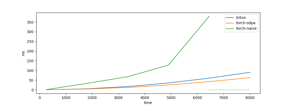
As expected, the Flash Attention algorithm completely outperforms the naive implementation performance-wise. Also, I've marked with a dashed line the range of lengths for which the naive implementation causes a CUDA out-of-memory error.
We see that our Triton implementation is slightly worse than PyTorch SDPA. But the difference is not too large Considering the fact that PyTorch SDPA is a well-optimized CUDA kernel, that's a nice result.
Benchmarking code is also available in the repository.

Conclusions
In the post, I covered the motivation of the Flash Attention algorithm as well as its algorithm details. Finally, we were able to implement it from scratch in Triton, reproducing the speedups from the paper.
I hope this post improved your understanding of Flash Attention. Feel free to leave a comment below if you have any questions.
References


