Training quantized neural networks typically involves two phases: full-precision (FP) pretraining followed by quantization-aware training (QAT). The conventional approach allocates about 10% of the training budget to QAT. But recent research at Apple shows this ratio is far from optimal, especially at scale.
In extreme cases, using the wrong QAT fraction can waste up to 50% of your compute budget. Moreover, what QAT bit-width should you pick given a fixed memory budget? Here's what we found after running ~800 experiments across different model sizes and training lengths.
The Resource Allocation Problem
When training QAT models, you face a fundamental trade-off: given a fixed compute budget, how should you divide training time between full-precision pre-training and quantization-aware training?
More FP training gives you a better starting checkpoint. More QAT training gives the model more time to adapt to quantization. Previous work (Liu et al., 2025) suggested 10% QAT was optimal but didn't explore how this changes with scale.
Key Observations
We trained models from 86M to 2.2B parameters across token counts ranging from billions to trillions, testing 1-bit through 6-bit QAT to see how performance changes.
The Optimal QAT Fraction Increases With Scale
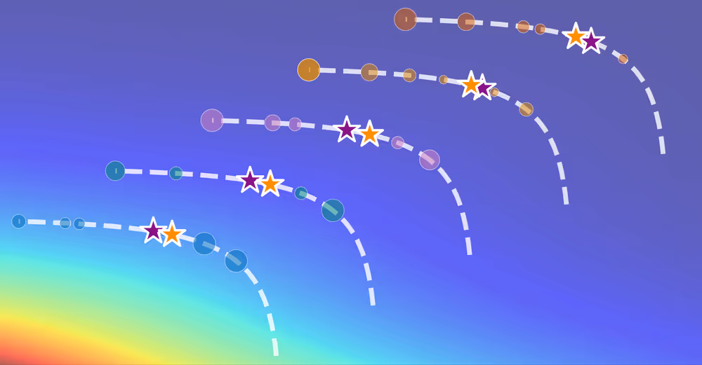
What we discover is that the optimal QAT fraction isn't fixed at 10%. It grows with your total compute budget, ranging from 10-15% for small-scale training to 55% or even more for large-scale training.
The intuition. Longer full-precision training packs more and more information in high-precision bits, making subsequent quantization harder. Therefore, the model needs more QAT steps to adapt to the precision loss. In fact, not just proportionally more steps but the portion itself starts to grow.
Predicting Optimal Fractions From Tokens-Per-Parameter-Byte
The optimal QAT fraction can be predicted using the tokens-per-parameter-byte statistic.
$$S_{\text{total}} = \frac{D_{\text{total}}}{N \cdot \frac{B}{8}},$$
where \(D_{\text{total}}\) is the total number of tokens, \(N\) is the parameter count, and \(B\) is the QAT bit-width. This metric captures several key insights:
- Larger models are easier to quantize (higher \(N\) → lower \(S_{\text{total}}\)
- Models trained longer are harder to quantize (higher \(D_{\text{total}}\) → higher \(S_{\text{total}}\))
- Lower bit-widths are harder to quantize (lower \(B\) → higher \(S_{\text{total}}\))
We achieve a low mean absolute error in predicting optimal QAT fractions across all experiments by using such a simple predictor:
$$\widehat{f}(D_\text{total}, N, B) = \frac{\exp\left(\log{S_\text{total}} - \frac{6.7297}{\log{S_\text{total}}}\right)}{S_\text{total}}.$$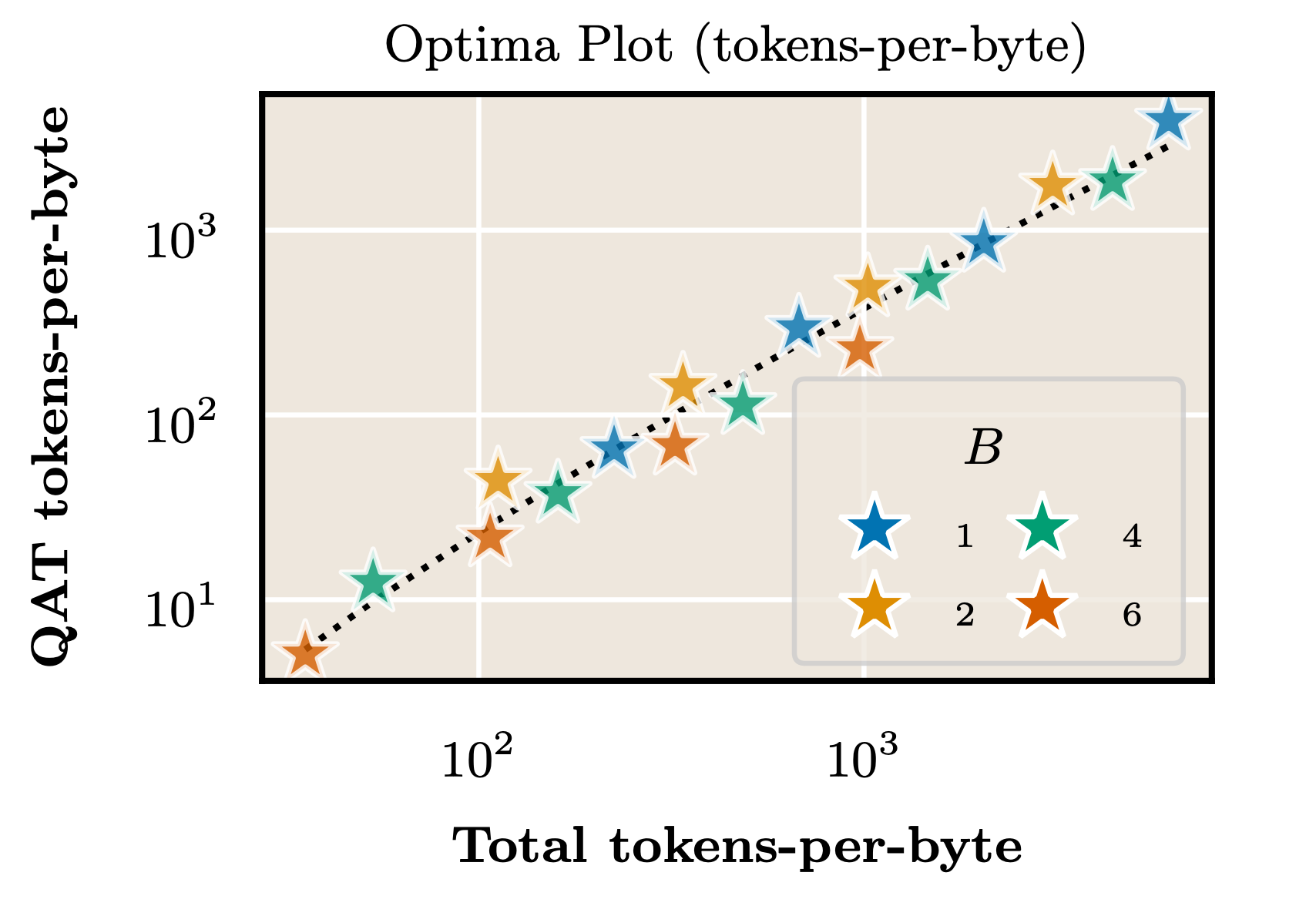
To capture full information, we can try predicting loss directly.
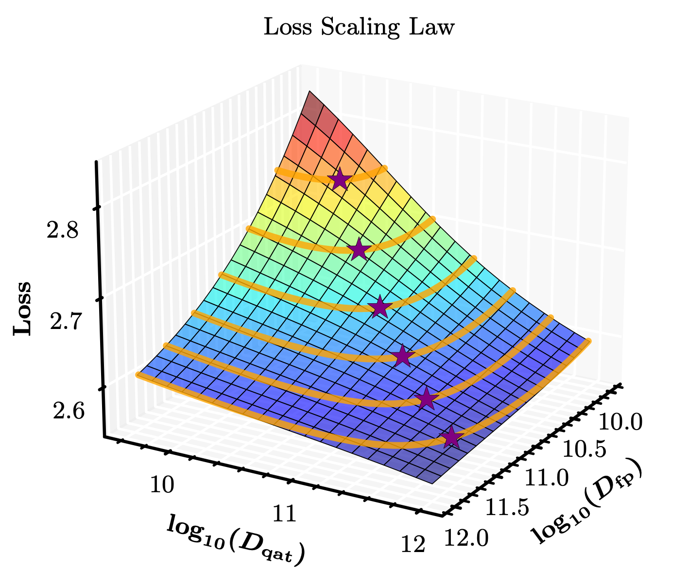
Loss Scaling Law
As noted, we moved to deriving a comprehensive loss scaling law that models final loss as a function of parameter count (\(N\)), full-precision tokens (\(D_{\text{fp}}\)), QAT tokens (\(D_{\text{qat}}\)), and bit-width (\(B\)). It not only predicts the final model's performance but also captures the observed phenomena of optimal QAT fraction:
$$L(N, D_\text{qat}, D_\text{fp}, B) = \underbrace{ \alpha + \frac{\beta}{D_{\text{total}}^{\gamma}} + \frac{\zeta}{N^{\eta}} }_{ \text{Chinchilla-like loss} } + \underbrace{ \delta(N, D_\text{qat}, D_\text{fp}, B) }_{ \text{QAT fraction-aware penalty} },$$ $$\delta(N, D_\text{qat}, D_\text{fp}, B) = \underbrace{ \theta \cdot 2^{- \kappa \cdot B}}_{ \text{Irreducible QAT error} } + \underbrace{ \frac{\phi \cdot 2^{- \chi \cdot B}}{N^{\psi} \cdot S_{\text{qat}}^{\omega}}}_{ \text{Pure QAT penalty} } + \underbrace{ \frac{\lambda \cdot 2^{- \mu \cdot B}}{N^{\nu} \cdot S_{\text{fp}}^{\xi} \cdot S_{\text{qat}}^{\rho}} }_{ \text{FP / QAT interaction} }.$$The QAT penalty term includes:
- Irreducible QAT error: Baseline penalty dependent on bit-width
- Pure QAT penalty: Loss that decreases with more QAT training
- FP/QAT interaction: Captures how FP training length affects QAT difficulty
The scaling law achieves $R^2 = 0.982-0.991$ across different bit-widths. Moreover, we can infer the optimal QAT fraction for a given compute by finding a minimum point with $D_\text{qat} + D_\text{fp} = const$. That's how the loss plot looks:
You can try exploring the scaling law through the following interactive plot:
Dfp Range
Dqat Range
Model Parameters
Drag to rotate • Scroll to zoom • Adjust sliders to explore the scaling law
Practical Predictions
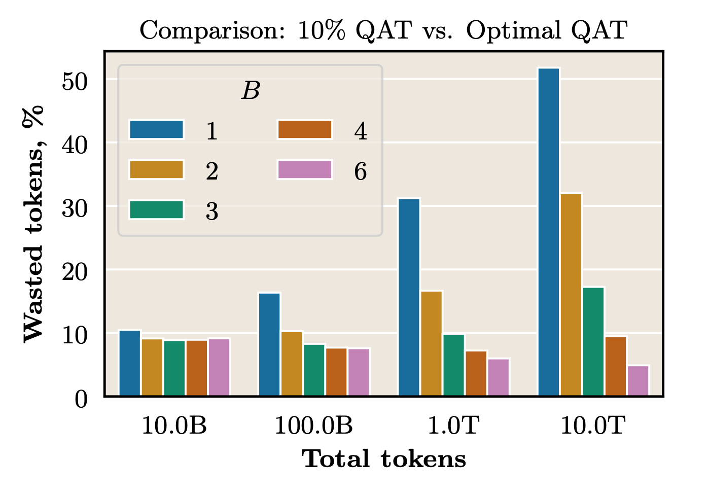
Ok, we know that there's an optimal QAT fraction, but how bad is a sub-optimal fraction? We can compare optimal and sub-optimal setups from the perspective of "wasted tokens" — how many more tokens you need to spend with a sub-optimal setup to match an optimal one.
Quantifying wasted compute
Using the fitted scaling law, we can quantify how bad a sub-optimal setup is. Comparing 10% QAT to optimal fractions reveals significant inefficiencies:
- 1-bit QAT: Up to 50% wasted tokens
- 2-4-bit QAT: 5-30% wasted tokens
- 6-bit QAT: 5-10% wasted tokens
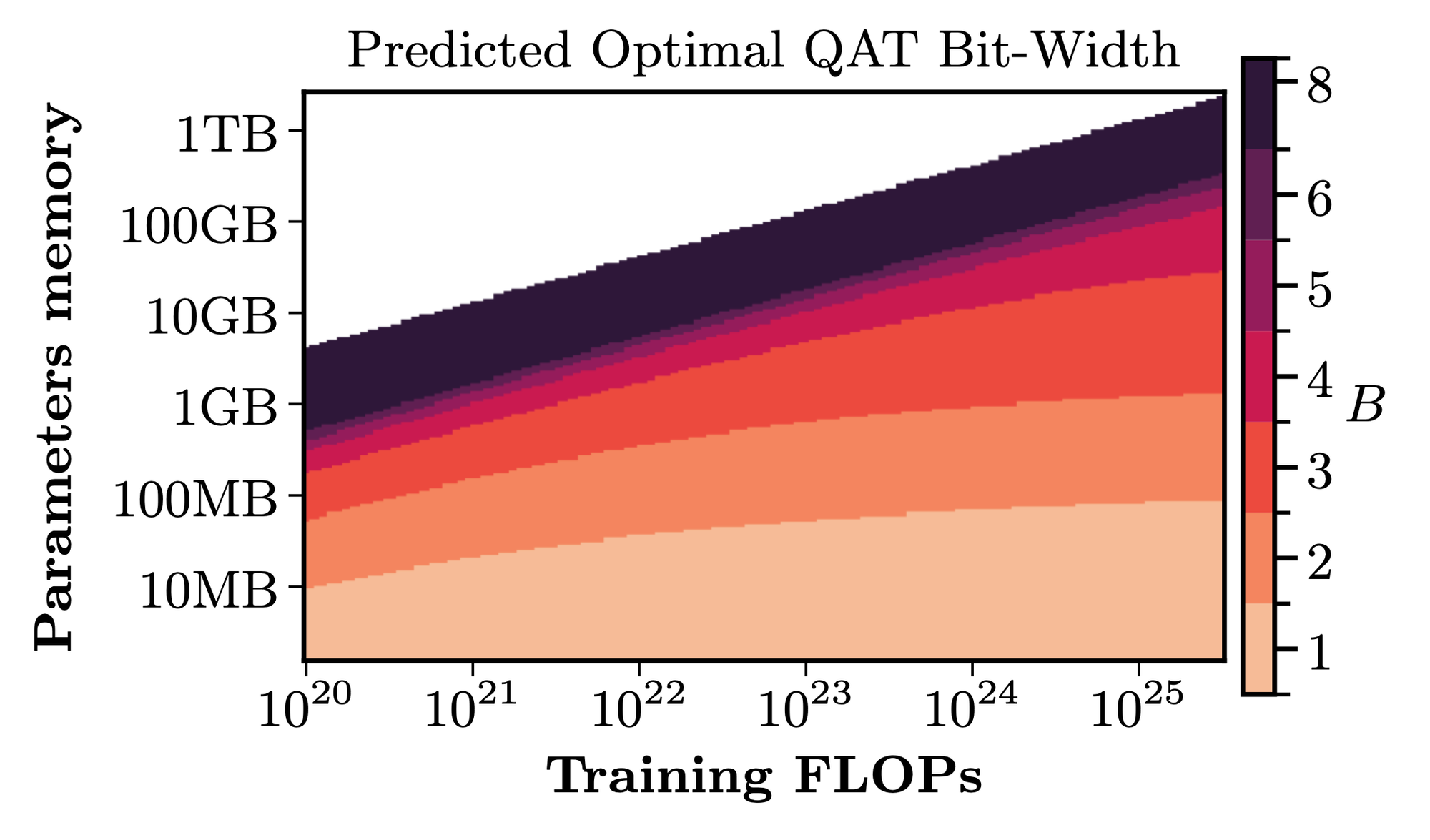
Optimal bit-width under memory constraints
Another useful use-case is inferring optimal QAT bit-width. Given a fixed memory budget, the scaling law determines whether you should use a larger model with lower bit-width or a smaller model with higher precision. The "fixed memory budget" is practically important as LLMs decoding is commonly bottlenecked by memory transfers. We found that optimal bit-width decreases as training compute increases.
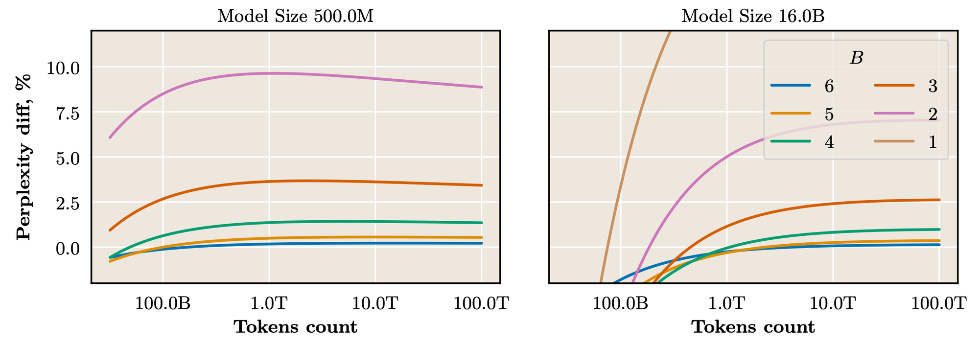
QAT accuracy vs full-precision
One perspective to plan QAT from is from the idea "when can we match full-precision performance?" The loss scaling law can help with that! We can compare each specific QAT bit-width for different token counts to full-precision performance. As expected, larger models tolerate lower bit-widths better, which has implications for choosing which bit-width to train.
Cooldown & QAT Fusion
Standard training performs learning rate cooldown on the full-precision model, then re-warms the learning rate for QAT. We speculate that those carefully adjusted weights during FP cooldown are almost discarded when quantization is initialized.
We propose cooldown & QAT fusion: skip the FP cooldown phase and perform learning rate decay jointly with QAT instead.
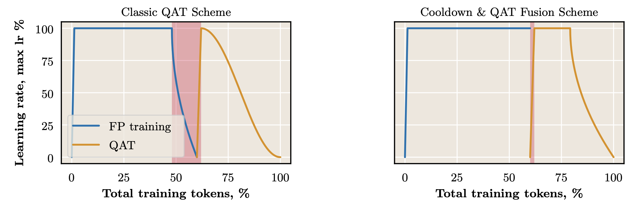
Results
QAT fusion shows good results on 4-bit and 6-bit QAT across different model sizes. We also experimented with lower bits, but gains there were not as evident. We believe this is because for lower bits, the optimal QAT fraction is quite high, which makes the effect from QAT fusion less noticeable.
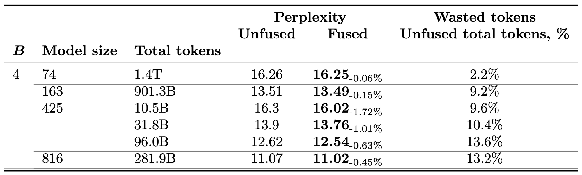
The perplexity improvements translate to billions of tokens' worth of compute saved.
Implementation Guidelines
If you're planning QAT, consider the following steps:
- Calculate tokens-per-parameter-byte and use it to predict optimal QAT fraction instead of assuming 10%.
- Budget compute appropriately — optimal fractions can exceed 50% for large-scale training.
- Implement cooldown & QAT fusion — it's a simple scheduler change with noticeable compute savings.
- Choose bit-width based on constraints — use the scaling law to optimize for your memory and compute budget.
- Pay extra attention to low-bit QAT — suboptimal fractions are much more costly for 1-2 bit quantization than 6-bit.
Conclusions
Efficient quantized model training requires careful compute allocation between full-precision and quantization-aware phases. The optimal QAT fraction isn't fixed—it increases with scale, from 10% to 50% or higher depending on tokens per parameter byte.
The loss scaling law enables us to:
- Predict optimal QAT fractions in advance
- Avoid significant compute waste (up to 50% for extreme cases)
- Select optimal bit-widths under memory constraints
- Achieve higher-quality quantized models for the same cost
Combined with cooldown & QAT fusion, these techniques provide substantial efficiency gains for training quantized models at scale. Full details and additional experiments are available in the original paper:
Work conducted at Apple with David Grangier, Angelos Katharopoulos, and Awni Hannun. All information is from the public paper preprint.
Apple and the Apple logo are trademarks of Apple Inc., registered in the U.S. and other countries and regions.